Google Earth Engine – Data Extraction Engine

The engine is designed to perform computations across large collections of polygons or points (features in GEE) over many images. The core idea is to disaggregate these computations into simple processes across a small set of features. In the default use case, we attempt to extract spectral values and derived spectral indices for all the forest pixels of Sentinel 1 raster files for the entire of Himachal Pradesh (state in India) for all months of 2024. The Sentinel 1 images are aggregated to monthly median images (one image for each month from January to August) and all pixels other than forest pixels are masked out.

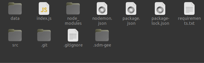
Please note the directory structure of GDEE as depicted below:

In order to perform the above computations, follow these detailed instructions:

1. Loading AOI

The state of Himachal Pradesh representing an area of 55,673 sq. Kms is the area of interest (AOI) which is initially loaded on the engine as a shape file comprising of only one polygon for the entire state. Users have two options to load the shape file:

a. **Upload the shape file as an asset to desired GEE account and call it in the `src/imageProcesses/sentinel1.js`**

    - Upload the shape file to the GEE account.
    - Import the shape file asset into `src/imageProcesses/sentinel1.js` using its asset ID.
    
b. **Save the shape file as a JSON file and store it in the directory `src/shp/hp_bounds.json`**

    - Convert the shape file to a GeoJSON format.
    - Save the GeoJSON file in the `src/shp/` directory with the name `hp_bounds.json`.
    - Load the JSON file as a Feature Collection on the engine by default.

State boundary of Himachal Pradesh (AOI) as single Polygon

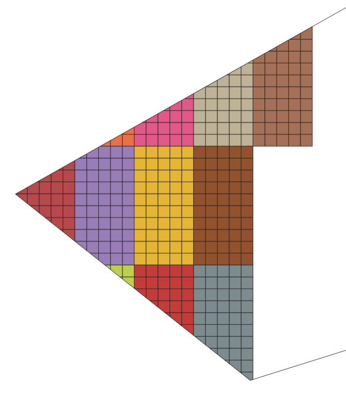
2. AOI Disaggregation – Creating Grids

The predefined AOI will split into two sets of fishnet grids. The user may create this as a separate process using any GIS software or GEE. The two sets of grids which are to be manually created are:

• a. Big grids – Fishnet grids of resolution 500 m by 1 km
• b. Small grids – Fishnet grids of resolution 100m by 100m

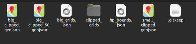
Both grids are to be clipped to the state boundary of Himachal Pradesh or the AOI. The clipped big grids should be stored as GeoJSON in the directory src/shp/big_clipped.geojson and clipped small grids as GeoJSON in the directory src/shp/small_clipped.geojson.

3. AOI Disaggregation – Grids Cross Clipping

We proceed to run the src/split_big_grids.py file by executing the command:

python src/split_big_grids.py

Snapshot of small grids (differentiated by black straight lines) inside big grids (differentiated by colors) clipped inside the AOI polygon

At the previously mentioned resolution of grids, we expect the number of small grids within each big grid to be not more than 50. This is a very stringent condition for ensuring low computation load and preventing a user memory limit. The maximum number of small grids within big grids can be increased if the raster to be processed is of a lower resolution. Currently we use Sentinel 1 which has a pixel resolution of 10 m. These cross clipped individual grids are later used in the processing of images sequentially so that computation load on the GEE server is low and doesn’t raise a “user memory limit” error.

Depending on the size of the AOI and the configuration of the local device, grids cross clipping can take a couple of days for successful execution. The default process lasted for 14 hours.

Snapshot of shp directory post grid clipping

As the grids cross clipping script executes, it creates a JSON file (shp/big_grids.json) that logs all the cross clipped grid JSON files stored in the local and uses the former to call the grids sequentially for processing.

4. Raster Processing

The directory src/imageProcesses contains the necessary scripts to call, preprocess, and initiate computations on each image. The sentinel1.js in the directory calls in the Sentinel 1 Image Collection from January 1, 2024, to August 31, 2024. The raster preprocessing involves the following:

• Clipping to AOI: The entire Sentinel 1 “ImageCollection” is filtered to the required data range and clipped to the AOI under consideration.
• Median Composites: The median composite of the clipped image collection for each month is computed using the default GEE function.
• Creating Spectral Indices: We use the various spectral bands of the images to create the necessary spectral indices and store them as new band values for each pixel.
• Masking: We use the ESA World Cover product to create crop, snow, water, and built-up area masks and apply them on the processed median composites.

5. Statistics and Computation

The engine will now initiate the src/utils/statsMaker.js to compute the necessary raster statistics for each clipped grid. In the default state, the script extracts spectral data for pixel bounds of the raster within the bounds of the clipped grid. The extracted values are then exported to the local device as CSV files.

If the user wants to perform any other computation on the raster for each grid, please update the src/utils/statsMaker.js script to achieve the same. The src/utils/localizeTable.js controls the process via which the values are downloaded and stored as files of the necessary format in the user’s local device. In the default state, the engine creates the data/download directory, which stores files in the following folder structure:

Users can alter or update this directory structure by making the necessary changes in the src/utils/createPaths.js script.

6. Initiate Engine

Initiate the engine instance by running the command:

npm start
In its default state, the engine starts with the express app log:
“Server is running on port 5000”.

6. API Call

In the default state, for extracting forest pixel values from Sentinel 1, the user must call the API, http://localhost:5000/sent1. Call the API using a web browser or a third-party client interface like ThunderClient. Post successful authentication, the data will be sequentially stored as CSV files in the data folder.